The notion of Machine Learning includes a wide group of statistical algorithms where a computer system learns on a set of training data and, after having completed its learning phase, uses its experience to generate predictions on new, unknown data. In the context of the capstone project of an advanced online training course at
EPF Lausanne, a swissbib admirer takes the challenge to do Machine Learning with a set of library catalogue data in MARC 21 format. The goal of the project is to build an artificial machine being capable to find duplicate records in the data. The project is done with three
distinct groups of models. In this blog, the results of a Decision Tree and a Random Forests model are presented.
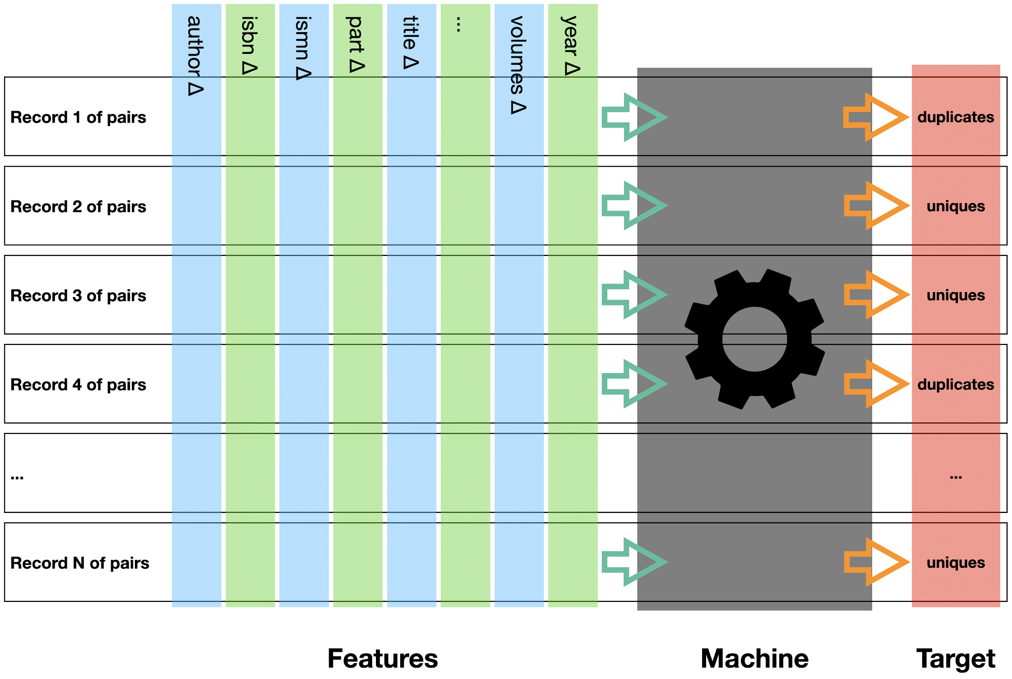
The starting point for Machine Learning is data. The data generally consists of two distinct types of variables, features and its target. The variables of the data set that serve as input for computing the prediction are called features. The features of the data are constructed with the help of two records of original swissbib data
containing raw information of a bibliographic unit, each. Such two records of raw data are paired in each of its attributes, calculating a numerical similarity distance for each pair of same attributes of the two bibliographical records, see
figure 1. For example, for two arbitrary records, the mathematical distance between title
1 (title of record r
1) and title
2 (title of record r
2) are determined to be the feature titleΔ =
sim(title
1,title
2), where
sim(x
1,x
2) is a mathematical similarity function. For the project at hand, twenty distinct similarities of two times twenty raw data attributes like title, author, year, ISBN, ISMN, etc. are calculated for each feature record. Therefore, the number of features are twenty. A feature record is represented as an array in the memory of a computer system. All rows of feature arrays can be represented in the form of
a
matrix. Therefore, the full set of this data is called feature matrix. The total of feature records used for training the data is nearly 260'000.
 |
| Figure 1: Records pairing |
The variable of a data set that is to be predicted by the machine is called output or target, see
figure 2. Each feature record has its target value. For each feature record of the project described above, the target variable indicates whether a data row of features is either a row of unique records or a row of duplicate records. The possible target values are 0 (row of unique records) or 1 (row of duplicate records), resp. A more detailed description on how to calculate the feature matrix and its array of target values for the training data will be given in a later blog to come.
 |
| Figure 2: Feature matrix, machine and target |
The idea behind a Decision Tree algorithm is that the computer system learns a set of sequential if-then-else rules that lead to a final decision. Each if-then-else statement is called a node of the Decision Tree. The nodes are arranged in sequences to form of a binary tree, see
figure 3, which is the reason for its naming. In the swissbib project, the set of if-then-else rules is a sequence of thresholds for binary statements of one feature variable that can either be lower or higher than the specific threshold. To classify a feature record, the algorithm starts at the top of the tree and evaluates the statement in each node on its path down. Depending on the threshold value, the algorithm decides for the right-lower or the left-lower node as the next node until reaching the bottom of the tree. The final decision is called a leaf of the Decision Tree. The leaf concludes the decision wether the feature record is a pair of uniques or a pair of duplicates. During training a Decision Tree, the if-then-else rules of the nodes are adjusted iteratively until the Decision Tree predicts the target value of the training data feature rows with the highest
possible probability according to a function to measure the quality of decisions, called criterion. When this highest power of prediction on the training data is reached, the Decision Tree can be used for predicting new, unseen data.
 |
| Figure 3: Graphical representation of the Decision Tree on swissbib data |
Decision Tree is a classical method of Machine Learning. Its advantage is its clarity. It can be easily interpreted when looking at the trained model tree. A Decision Tree classifier can be built with the help of different parameters. In the project, the varied parameters are the maximum depth of the tree as well as the so called criterion, the mathematical function to measure the quality of a split in the nodes. Several specific Decision Trees are calculated with the help of
cross-validation and their prediction power is compared. The project finds the best Decision Tree for swissbib data to have a maximum depth of 26 nodes and a criterion of
Gini impurity.
The performance of a Machine Learning classifier can be measured with the help of some metrics derived from the confusion matrix, see
figure 4. The confusion matrix compares the predictions of a trained machine on some validation data with their given target values. Four cases can be distinguished.
- Two "true" cases (1. "true positive" and 2. "true negative") according to the two specific classes are the correctly predicted records of the validation data.
- Two "false" cases (3. "false positive" and 4. "false negative") according to the two specific classes are the wrongly predicted records of the validation data.
 |
| Figure 4: Confusion matrix |
From the four cases above, a metrics called
accuracy can be calculated, allowing a statement on the prediction quality of the model on unknown data. For swissbib's calculated Decision Tree, an accuracy value of nearly 99.95% can be reached. This accuracy means 27 wrongly predicted records on a total of 51'886 validation records.
For comparison reasons, a
Random Forests model is calculated additionally. A Random Forests is an Ensemble method. It consists of an ensemble of Decision Trees that are assembled during the learning phase. Again, the set of best parameters for the Random Forests is searched for swissbib data and a number of 100 trees of maximum depth of 22 each in the forest is found to generate the best results. With Random Forests, an accuracy of nearly 99.95% can be reached, too, with the same total of wrongly predicted records of 27 on the total of the validation records.
The project is implemented in programming language
Python, using library
scikit-learn for calculating the models. The Random Forests implementation of this library allows for assessing the importance of each feature for prediction.
Figure 5 shows the normed importance value of the features used. It can be seen that variable year is the leading variable for indicating wether a pair of records is a pair of uniques or of duplicates. Variable title is the second most important feature for the Random Forests model, but also author and volumes indication are of high relevance. The importance of features like coordinate and ISMN seem to be low. This is due to the fact that only few of swissbib's raw data are of format map of music. Therefore, only few of swissbib's raw data hold any information in these attributes.
 |
| Figure 5: Normed feature importance of Random Forests |
The results presented here, suggest swissbib to implement a new deduplication process with the help of a Random Forests algorithm, due its best overall performance on the training data. The project described here, implements some more models different to the Decision Tree and the Random Forests models. The results of those will be presented in some additional blog articles (see
here).


